Análisis de datos de conteo en ecología

B0305 – Lab Eco Gral
https://ucr-ecologia.github.io/B0305-lab-eco-gral/

Prof. Teo Nakov

Escuela de Biologia, Universidad de Costa Rica

04 Sep 2025

¿Qué son los Datos de Conteo?

Definición: Números enteros no negativos que representan el número de ocurrencias de un evento
Rango: 0, 1, 2, 3, 4, …
No pueden ser negativos ni fraccionarios

¿Por qué tratamiento especial?

Discretos, no continuos
Distribuciones a menudo sesgadas
La varianza a menudo está relacionada con la media

Datos de Conteo en Biología y Ecología

Ejemplos comunes:

Número de especies en un cuadrante
Semillas por fruto
Parásitos por hospedero
Descendencia por individuo
Visitantes a flores por hora
Cajas nido ocupadas por sitio

¿Por qué esto importa?

¡Las distribuciones normales y modelos lineales pueden no ser apropiados!

La Distribución de Poisson

La distribución “por defecto” para datos de conteo

Parámetro: λ (lambda) = media = varianza
Supuesto: los eventos ocurren independientemente

Propiedad clave: La media es igual a la varianza

Si media = 3, entonces varianza = 3
Esto a menudo se viola en datos ecológicos

Problemas con Datos de Conteo Ecológicos

Dos problemas principales:

Sobredispersión - varianza > media
Inflación de ceros - más ceros de los esperados

¿Por qué ocurren en ecología?

Sobredispersión: Agregación espacial, heterogeneidad ambiental, variables no medidas
Inflación de ceros: Ausencias verdaderas vs. fallas de detección, idoneidad del hábitat

Sobredispersión en Detalle

¿Qué es?

La varianza excede la media
Indica variabilidad extra no capturada por Poisson

Causas en ecología:

Agregación espacial (organismos se agrupan)
Heterogeneidad ambiental
Diferencias individuales en rasgos
Covariables no medidas

Consecuencias estadísticas:

Errores estándar subestimados
Valores p artificialmente pequeños
Incremento en tasas de error Tipo I (encontrar diferencias que no existen)
Conclusiones excesivamente confiadas

Errores Tipo I y Tipo II

Recordatorio: Tipos de Error Estadístico

Realidad vs Decisión	No rechazar H₀	Rechazar H₀
H₀ es verdadera	✓ Correcto	❌ Error Tipo I
H₀ es falsa	❌ Error Tipo II	✓ Correcto

Error Tipo I (α): Rechazar H₀ cuando es verdadera (“falso positivo”)
Error Tipo II (β): No rechazar H₀ cuando es falsa (“falso negativo”)

En contexto de sobredispersión: Ignorar la sobredispersión eleva Error Tipo I

Evaluando la Sobredispersión

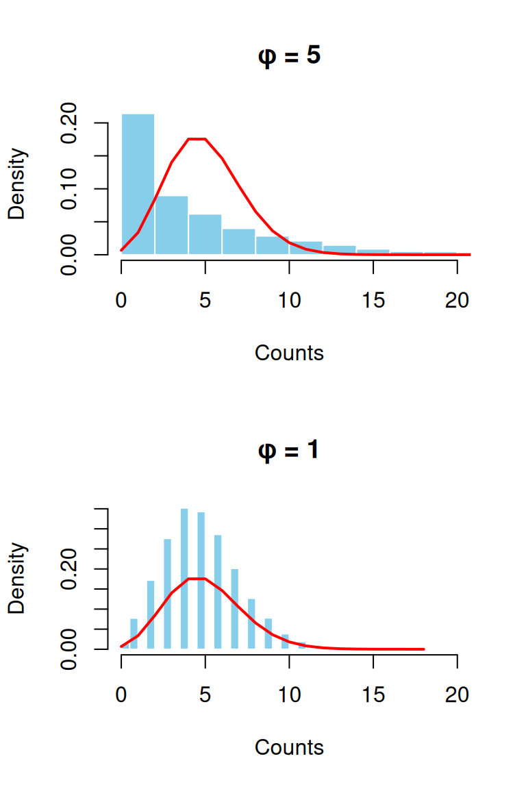
Paso 1: Calcular parámetro de dispersión

φ = Devianza residual / Grados de libertad residuales
φ ≈ 1: Poisson es adecuado
φ > 1: Sobredispersión presente

Paso 2: Pruebas formales

LRT: Comparar Poisson vs. Binomial Negativa
AIC/BIC: Criterios de información para selección de modelos

Ejemplo: Peligro de Ignorar la Sobredispersión

Código R:

# Simular datos sobredispersos
set.seed(123)
library(MASS)

# Generar datos con NB
# (media=5, sobredispersión)
counts <- rnegbin(40, mu = 5, theta = 1)

# Dividir en 2 "hábitats" aleatoriamente
habitat <- rep(c("Mar", "Rio"), each = 20)
data <- data.frame(counts, habitat)

# Modelo Poisson (INCORRECTO)
m_poisson <- glm(counts ~ habitat, 
                 family = poisson, data = data)

summary(m_poisson)


Call:
glm(formula = counts ~ habitat, family = poisson, data = data)

Coefficients:
            Estimate Std. Error z value Pr(>|z|)    
(Intercept)  1.67710    0.09667   17.35   <2e-16 ***
habitatRio  -0.35534    0.15060   -2.36   0.0183 *  
---
Signif. codes:  0 '***' 0.001 '**' 0.01 '*' 0.05 '.' 0.1 ' ' 1

(Dispersion parameter for poisson family taken to be 1)

    Null deviance: 232.43  on 39  degrees of freedom
Residual deviance: 226.78  on 38  degrees of freedom
AIC: 333.12

Number of Fisher Scoring iterations: 6

# Verificar sobredispersión
deviance(m_poisson) / df.residual(m_poisson)

[1] 5.967796

Modelo Binomial Negativa (CORRECTO)

m_nb <- glm.nb(counts ~ habitat, data = data)
summary(m_nb)


Call:
glm.nb(formula = counts ~ habitat, data = data, init.theta = 0.825913691, 
    link = log)

Coefficients:
            Estimate Std. Error z value Pr(>|z|)    
(Intercept)   1.6771     0.2644   6.344 2.24e-10 ***
habitatRio   -0.3553     0.3792  -0.937    0.349    
---
Signif. codes:  0 '***' 0.001 '**' 0.01 '*' 0.05 '.' 0.1 ' ' 1

(Dispersion parameter for Negative Binomial(0.8259) family taken to be 1)

    Null deviance: 45.513  on 39  degrees of freedom
Residual deviance: 44.637  on 38  degrees of freedom
AIC: 213.93

Number of Fisher Scoring iterations: 1

              Theta:  0.826 
          Std. Err.:  0.231 

 2 x log-likelihood:  -207.925

Lección

Mismo coeficiente, pero error estándar realista → conclusión correcta

Inflación de Ceros en Detalle

¿Qué es?

Más ceros observados que los predichos por Poisson (o Binomial Negativa)

Dos tipos de ceros:

Ceros estructurales: Ausencias “verdaderas” (hábitat no adecuado)
Ceros de muestreo: Presente pero no detectado

Ejemplos:

Conteos de peces en arroyos (algunos sitios no adecuados para peces)
Cargas parasitarias (algunos hospederos resistentes)
Conteos de plantas (algunas parcelas carecen de condiciones adecuadas)

Evaluando la Inflación de Ceros

Evaluación visual:

Comparar conteos de ceros observados vs. esperados
Histograma de la distribución de datos

Pruebas formales:

LRT: Modelos con inflación de ceros vs. estándar
AIC/BIC: Comparación de criterios de información

Regla práctica:

Si >60-70% son ceros, considerar modelos de inflación de ceros

Ejemplo: Cuándo Usar Modelos Zero-Inflated

Código R:

# Simular peces en Mar vs. Río
set.seed(456)
library(pscl)

# Generar datos zero-inflated
n <- 40
habitat <- rep(c("Mar", "Rio"), each = 20)

# Crear inflación de ceros estructural
# Mar: más peces, Rio: muchos ceros
prob_zero <- ifelse(habitat == "Rio", 0.7, 0.2)
counts <- ifelse(runif(n) < prob_zero, 0,
                 rpois(n, lambda = 8))

data <- data.frame(counts, habitat)

Datos observados:
- 65% de ceros (mucho más que Poisson)
- Mar: Pocos ceros, conteos altos
- Río: Muchos ceros (condiciones no aptas)

Modelos

Modelo Binomial Negativa:

m_nb <- glm.nb(counts ~ habitat, data = data)
summary(m_nb)


Call:
glm.nb(formula = counts ~ habitat, data = data, init.theta = 1.236507457, 
    link = log)

Coefficients:
            Estimate Std. Error z value Pr(>|z|)    
(Intercept)   1.9315     0.2184   8.845   <2e-16 ***
habitatRio   -0.6232     0.3188  -1.955   0.0506 .  
---
Signif. codes:  0 '***' 0.001 '**' 0.01 '*' 0.05 '.' 0.1 ' ' 1

(Dispersion parameter for Negative Binomial(1.2365) family taken to be 1)

    Null deviance: 54.486  on 39  degrees of freedom
Residual deviance: 50.687  on 38  degrees of freedom
AIC: 222.98

Number of Fisher Scoring iterations: 1

              Theta:  1.237 
          Std. Err.:  0.443 

 2 x log-likelihood:  -216.979

Modelo ZINB (correcto):

m_zinb <- zeroinfl(counts ~ habitat | habitat, dist = "negbin", data = data
)
summary(m_zinb)


Call:
zeroinfl(formula = counts ~ habitat | habitat, data = data, dist = "negbin")

Pearson residuals:
     Min       1Q   Median       3Q      Max 
-1.92830 -0.95007  0.02794  0.84733  2.38795 

Count model coefficients (negbin with log link):
            Estimate Std. Error z value Pr(>|z|)    
(Intercept)  2.03622    0.08925  22.815   <2e-16 ***
habitatRio  -0.13161    0.15079  -0.873    0.383    
Log(theta)   4.39992    3.36360   1.308    0.191    

Zero-inflation model coefficients (binomial with logit link):
            Estimate Std. Error z value Pr(>|z|)   
(Intercept)  -2.2039     0.7499  -2.939  0.00329 **
habitatRio    1.9997     0.8747   2.286  0.02224 * 
---
Signif. codes:  0 '***' 0.001 '**' 0.01 '*' 0.05 '.' 0.1 ' ' 1 

Theta = 81.4445 
Number of iterations in BFGS optimization: 23 
Log-likelihood: -91.42 on 5 Df

Interpretación:


Call:
zeroinfl(formula = counts ~ habitat | habitat, data = data, dist = "negbin")

Count model coefficients (negbin with log link):
(Intercept)   habitatRio  
     2.0362      -0.1316  
Theta = 81.4445 

Zero-inflation model coefficients (binomial with logit link):
(Intercept)   habitatRio  
     -2.204        2.000

Ríos tienen 7x más probabilidad de ser ceros estructurales (exp(1.99) ≈ 7.3)
Dado que hay peces presentes, no hay diferencia significativa en abundancia entre habitats

Lección

ZINB permite separar presencia/ausencia vs. abundancia dado presencia - dos procesos biológicos distintos

Comparación de Modelos

Modelo	Cuándo usar	Pregunta típica	Ventaja principal	Desventaja principal
Poisson	Media ≈ varianza Sin exceso de ceros	¿Cómo afecta X la abundancia?	Sencillo e interpretable	Asume equidispersión (rara en ecología)
Binomial Negativa	Sobredispersión presente	¿Qué factores afectan abundancia con variabilidad realista?	Maneja sobredispersión Interpretación similar a Poisson	No maneja inflación de ceros
ZIP/ZINB	Exceso de ceros ± sobredispersión	¿Qué determina presencia vs. abundancia?	Modela dos procesos biológicos distintos	Más complejo Requiere justificación biológica

Selección de Modelos

Criterios de información:

AIC: Criterio de Información de Akaike (más tolerante a la complejidad del modelo)
BIC: Criterio de Información Bayesiano (más conservador, tiende a favorecer modelos simples)
Valores menores indican mejor ajuste

LRT:

Solo para modelos anidados
OK: Poisson vs. Binomial Negativa ✓, ZIP vs. ZINB ✓
NOT OK: Poisson vs. ZIP ✗, Poisson vs. ZINB ✗, Binomial Negativa vs. ZINB ✗ (no anidados)

Leer más sobre AIC

Burnham, K.P. & Anderson, D.R. (2002). Model Selection and Multimodel Inference: A Practical Information-Theoretic Approach

Interpretación de Resultados

Coeficientes Poisson/Binomial Negativa:

Coeficiente crudo: Cambio en log(media) por incremento unitario
Coeficiente exponenciado: Cambio multiplicativo en la media
exp(β) = 1.5 significa incremento del 50%

Ejemplo:

β = 0.405 → exp(0.405) = 1.5
“Un incremento unitario en X se asocia con incremento del 50% en el conteo esperado”

Recordar

Siempre reportar intervalos de confianza - La incertidumbre es parte fundamental del resultado

Resumen

Mensajes clave:

Los datos de conteo requieren tratamiento estadístico especial
Verificar sobredispersión e inflación de ceros
Empezar simple, agregar complejidad según sea necesario
La selección de modelos es crucial
Interpretar resultados en contexto biológico

Recordar:

Los modelos son herramientas, no verdades
Los supuestos importan
El entendimiento biológico guía las decisiones estadísticas

Bibliografía

Gotelli, N.J. & Ellison, A.M. (2004). A Primer of Ecological Statistics. Sinauer Associates.

Recursos adicionales:

Burnham, K.P. & Anderson, D.R. (2002). Model Selection and Multimodel Inference: A Practical Information-Theoretic Approach. 2nd ed. Springer-Verlag.
Zuur, A.F., Ieno, E.N., Walker, N.J., Saveliev, A.A. & Smith, G.M. (2009). Mixed Effects Models and Extensions in Ecology with R. Springer.
Bolker, B.M. (2008). Ecological Models and Data in R. Princeton University Press.